

Practical PID Process Dynamics with Proportional Pressure Controllers
Category:
Rationally minded design engineers understand the importance of competent controls engineers when it comes time to implement their designed process. After spending months or years designing, specifying, and securing the necessary equipment, design engineers must trust the controls engineer to complete the vision and automate a repeatable process. While the collaboration between engineering disciplines continues imperatively, design engineers who develop a practical understanding of PID loop control are best positioned to specify and secure optimal equipment, which improves the probability of successful implementations and may significantly reduce the time to return on investment.
Every time we modify our behavior based on a previous result, we create a control loop. As humans, we continually form new control loops and tweak old ones in an attempt to regulate our experience. We adjust the speed of our vehicles by varying fuel input based on speedometer readings. We walk outdoors, sense the temperature, and add or subtract clothing to create comfort. The human brain is the most prolific loop controller in existence. Naturally, we implement similar techniques to control our manufacturing and industrial processes.
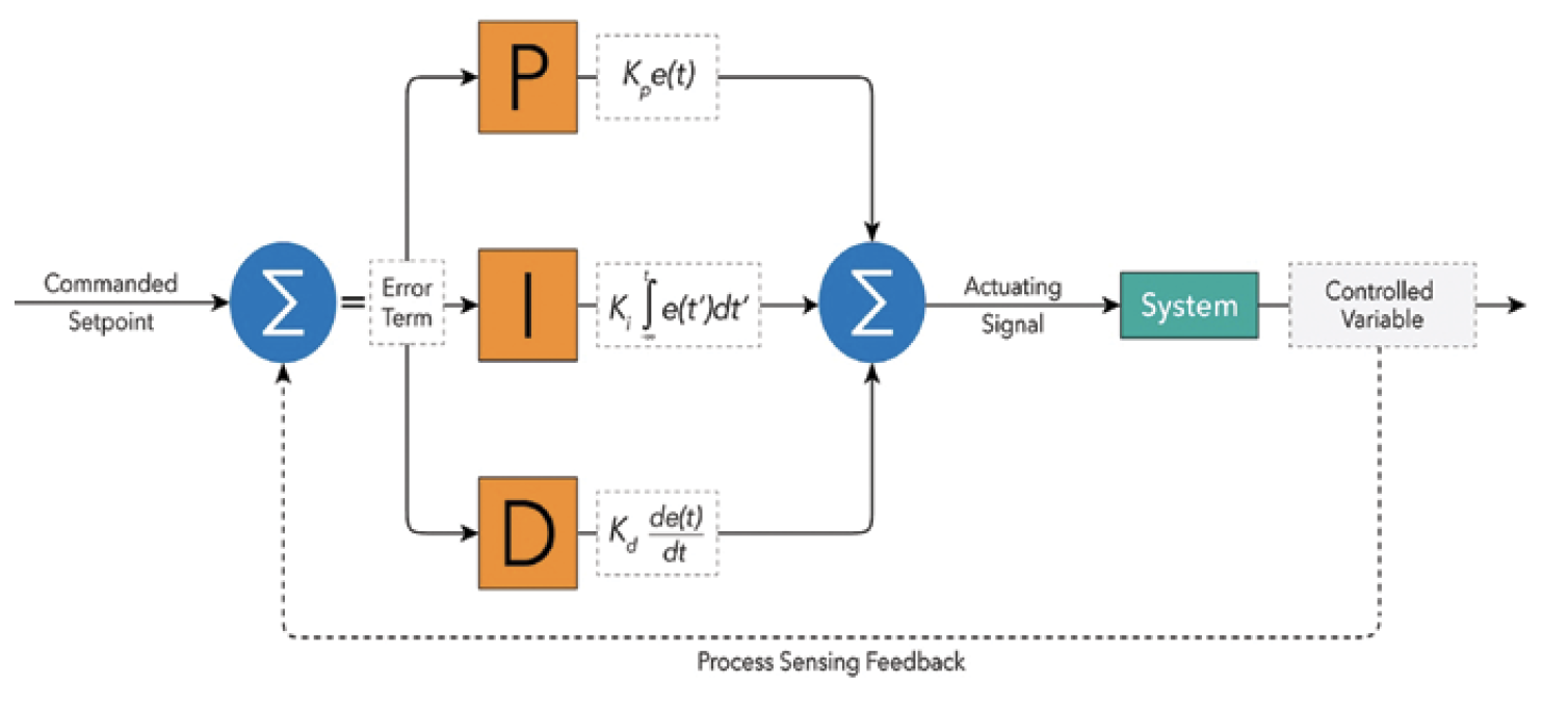
The vast majority of industrial control loops utilize some combination of PID control. PID is an acronym for Proportional, Integral, and Derivative. These mathematical terms reference algorithms that controls engineers use to manipulate actuation signals to achieve desired process results. Industrial process loops incorporate multiple sensors and various valves, cylinders, or other devices requiring actuation. Typical PID loop utilization includes temperature, pressure, flow rate, chemical composition, speed, and level. A controls engineer utilizes PID algorithms to record process data and calculate setpoints to various actuation devices. The challenge is to overcome numerous variables and reach the desired setpoint at the correct time with minimal over or undershoot.
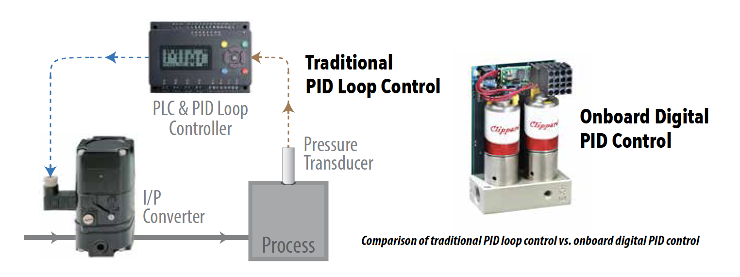
A common component in many control loop processes is the proportional controller. This device requires a setpoint from a master controller with the expectation it generates an equal output. The master controller may utilize PID loop control to calculate a setpoint to the proportional controller. However, modern proportional controllers have incorporated their own onboard adjustable PID loop to achieve the commanded setpoint.
It is within the context of proportional controllers that this paper explores and discusses practical PID process dynamics.
By understanding basic PID theory and behavioral tendencies, design engineers are equipped to appreciate the nuances and priorities of each specific process and select optimal proportional controllers. Speed, accuracy, resolution, and stability influence each other, and each one is affected when PID settings are modified. Which one is most important? Analog proportional controllers are fast, but do microcontroller-based devices offer any advantage? Is it possible for a proportional controller to provide flexibility and performance?
Proportional, Integral, and Deriviative Tendencies
PID loops give controls engineers a customizable method to control numerous conditions, from speed to temperature and everything in between. The loop's authority modifies device behaviors to maintain stable output and improve response rates. The most common proportional controllers are electronic pressure regulators (EPRs) consisting of fill and exhaust valves, an onboard transducer, and PID controls to adjust response performance. EPRs only require an external setpoint command to become a closed-loop control scheme. The setpoint is continually compared against the onboard transducer to produce an "error term." The singular intent of industrial PID control loops is to reduce and maintain the error term at or near zero at all times. So, how does each algorithm contribute to this goal?
The Proportional Algorithm Contribution
As the first ingredient in our control loop, the proportional algorithm is generally the most impactful and most crucial of the three. The P component is responsible for adjusting the control variable proportionally to the amount of calculated error in the process. The calculation for P output is simple: 'present-error' x Kp (proportional gain constant). Adjusting the P-gain value increases or decreases the rate of response. Some processes employ a P-only control scheme. However, if the proportional algorithm is the only element engaged in a system, stable operation can occur, but a steady-state error persists, and oscillation may become inherent in the process.
Consider the analogy of quadcopter drones. These aircraft utilize complex PID algorithms that use onboard sensor data to calculate the speed motors should spin to maintain the aircraft's desired position. In this example, the P algorithm is the responsiveness and sensitivity setting, and it determines how vigorously the controller works to correct the error. Generally speaking, a low P setting feels soft and sloppy on the controls, and a high P setting feels sharp and snappy. However, if the P setting is too high, it over-corrects and overshoots the setpoint, creating high-frequency oscillations. These oscillations can be reset and biased out manually, but to automatically eliminate the steady-state error inherent with oscillations, the integral must contribute its function to the control scheme.
The Integral Algorithm Contribution
The integral is the aggregate of all recorded values, from the time counting begins until the time counting stops. The I component records all errors above or below zero error (compared to the setpoint) and continually strives to reduce it to zero or near zero. Since the integral compiles errors over time, it removes any steady-state error in the system. Whereas the P reacts instantaneously to counterbalance for error at a specific point in time, the I compensates for all error across all known time. The integral calculation is 'accumulated-error' x Ki (integral gain constant).
As it relates to the quadcopter, the integral setting is most consistent with the feel of stiffness. It is responsible for maintaining drone altitude against external forces, such as wind or additional weight. If a steady wind is blowing, the I component produces an ever-increasingly stable altitude as the accumulation of historical error is averaged and implemented. However, if an unexpected gust of wind occurs, the I response may not be sufficient to compensate, and the derivative algorithm activates.
Graph of the integral
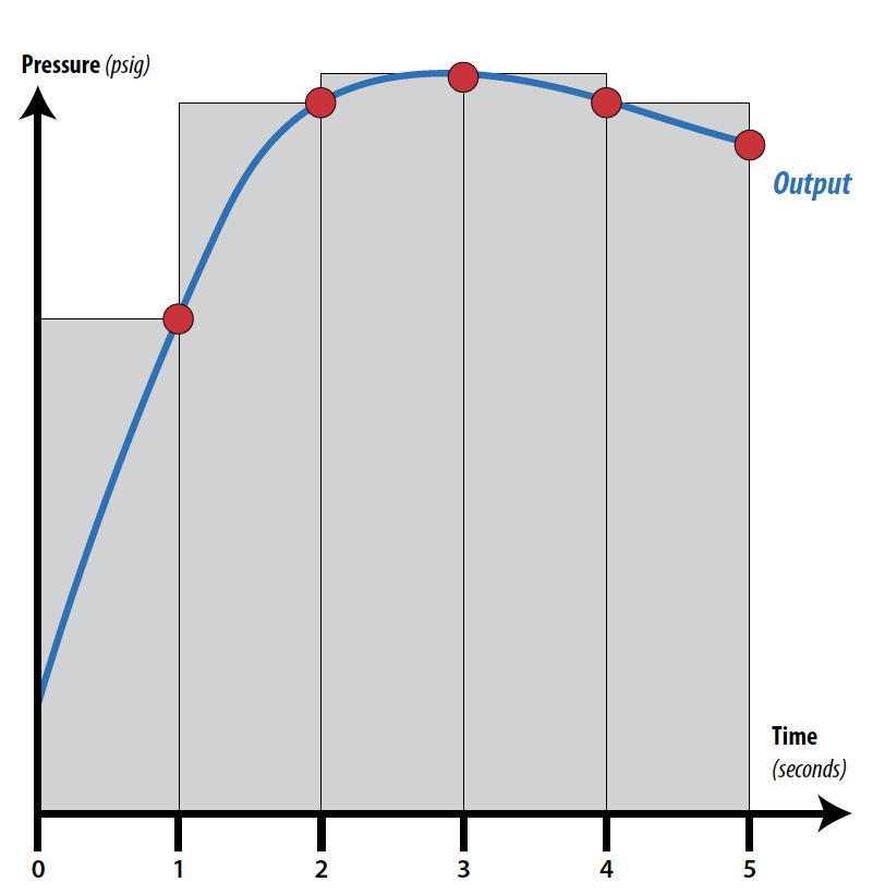
The integral is the aggregate of all recorded values, from the time counting begins until the time counting stops.
The Derivative Algorithm Contribution
If the proportional is the present-error correction and the integral is the past-error correction, then the derivative is the future-error correction. The D component is the most complicated and is usually unnecessary in most applications. In fact, most proportional controllers employ a PI control loop only. However, D action is beneficial in motion control applications as it is concerned with the instantaneous rate of change (derivative) in the recorded error. If there is no change in error, the derivative output is zero. If the rate of change increases or decreases, a derivative output occurs, one that corresponds to the magnitude of the instantaneous change in error. The D contribution is most effective when the P and I contributions are small. In this state, if the error spikes, the P and I components may take too long to react. However, the spike is what the D component is looking for, and thus, it reacts and compensates immediately. The derivative calculation is 'derivative-of-error' x Kd (derivative gain constant).
If a significant gust of wind hits the drone, the derivative action activates to compensate for the sudden rate change in error. The D output attempts to dampen over-correction from the P component by softening and neutralizing excessive P output action. Most closed-loop industrial processes do not consistently experience situations requiring D action; thus, a PI controller is most commonly employed.
Simple PI Troubleshooting
The drone analogy above is relatable because it references feelings and sensations that everyone understands. However, a controls engineer does not "feel" the temperature rising or "sense" a pressure drop; they use raw data and graphing tools to map sensor readings and compare against setpoints.
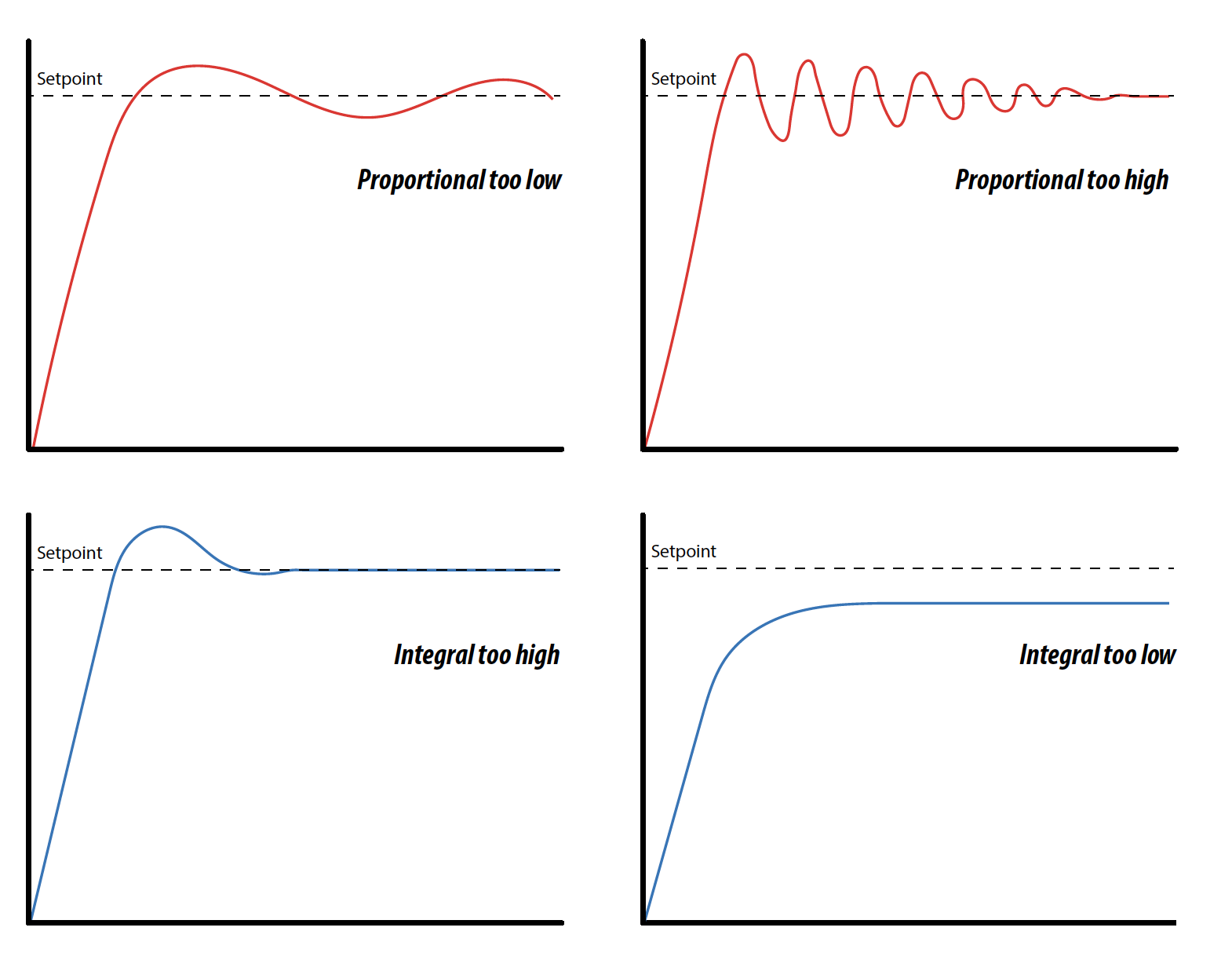
When tuning PI control loops, much trial and error is necessary to dial in the settings. For this reason, tuning PI loops is as much an art form as it is science. The graphs below show typical PI behaviors experienced with proportional controllers and the recommended action to tune them out.
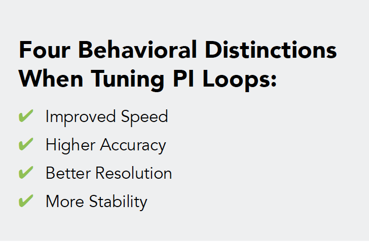
Know Your Process Priorities
When discussing proportional controller applications and how pressure controls perform, there are four behavioral distinctions to be aware of when tuning PI loops for optimal performance. Depending on the process, an electronic pneumatic controllers may need improved speed, higher accuracy, better resolution, or more stability. The question is: what is the priority for a particular process?
For example, traditional saturated steam temperature control requires good accuracy with stable temperatures. However, this cannot be achieved quickly for multiple reasons. A typical setup includes a thermocouple measuring downstream temperature and a PI controller calculating a setpoint to a process valve (proportional controller) based on temperature readings from the thermocouple. Since the proportional controller is merely opening and closing a valve to allow more or less steam downstream, temperature continuously dithers up and down around the desired setpoint. Eventually, the downstream temperature equals the setpoint, but the process necessitates 45 minutes to an hour. Sacrificing speed to achieve stable and accurate temperatures remains a priority for many steam temperature applications.
How does knowing the priorities of a process empower design engineers to specify optimal equipment?
Speed is the parameter that influences the other parameters the most. The faster a process needs to be, the more challenging it is to maintain accuracy, resolution, and stability. By understanding the irrelevance (from a physics and technology perspective) of speed in steam temperature control, a smaller (Cv) process valve could be selected, leaving more budget for a higher quality thermocouple.
What if speed wasn't constant and predictable adjustments would occur?
For example, microfluidics is a process designed to transport individual cells through microscopic channels for a diverse spectrum of analysis objectives—delivering stable speeds is imperative. However, a slow controlled speed is frequently preferred. Electronic pressure regulators (EPRs) are often employed to control the pressure of various fluids, each with different viscosities, densities, and other dissimilar attributes. If process variables like fluid, pressure, and volume change, PI settings require retuning for optimal performance.
Many pressure regulators work well when tuned correctly, but is it easy to modify PI settings when parameters change? Both digital and analog proportional controllers are available, should one technology be preferred over the other?
The short answer is yes! Controls engineers do prefer one of these technologies, and soon design engineers will too.
Comparing Digital vs. Analog PID Control
Analog Proportional Controller
Advantages and Limitations
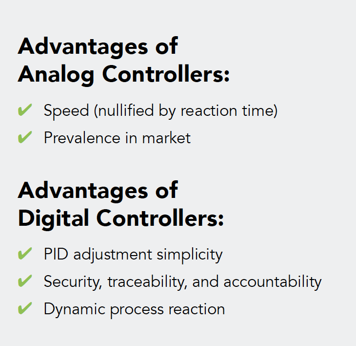
Analog proportional controllers possess two potential advantages over digital (microcontroller) based devices. First, the speed of analog circuits is faster than digital circuits. However, this is irrelevant to proportional controllers because no matter how fast an electrical signal opens or closes a valve, the fluid traversing the valve is always slower to react, nullifying the perceived advantage. Second, analog technology is prevalent in the market and requires less of a learning curve to implement and operate. While potentially a current advantage, the trend is clearly towards digital. Both advantages mentioned only highlight the vacuum of a single analog advantage relevant to this paper: PID control.
Digital PID Control Advantages
Understanding the digital versus analog preference comes down to understanding the particular control technology a device employs. Is the circuitry analog, or is a microcontroller onboard governing the operation of the device? While the market prevalence of analog devices can make selecting analog equipment a default decision, digital proportional microcontrollers offer numerous improvements over their analog counterparts, particularly in the context of enhanced PID functionality.
General PID-Loop Schematic Structure
PID Adjustment Simplicity
Tuning PID settings on some analog electronic pressure regulators is a tedious and time-consuming process requiring an operator to rotate tiny potentiometers manually. However, modifying digital PID parameters is accomplished through a simple software interface allowing the operator to directly manipulate settings via keyboard until the device reaches the desired performance characteristics. This one difference is enough to excite any controls engineer and curtail hours of labor.
Security, Traceability, and Accountability
PID security is an added benefit of microcontroller managed devices. When the factory-tuned PID settings produce undesired process performance, operators may tamper with the analog controller's PID potentiometers, creating additional issues. Once the PID settings are modified, it is challenging to return the device to initial calibration. However, Microcontroller PID changes require a software interface that retains all the revisions to the PID settings, producing accountability, and making it simple to return to factory settings if the new values perform poorly.
Dynamic Process Reaction
In the world of electronic pressure regulators (EPRs), some applications are static, demanding only simple pressure control in a closed volume. However, numerous applications are dynamic with varying setpoints, inlet pressures, volumes, back pressures, and leaks. Discovering PID values that keep an analog pressure control well-behaved during dynamic conditions is difficult, if not impossible. A proportional microcontroller can change PID values any time through a technique called gain scheduling where the microcontroller selects new values based on real-time variations (triggers) in operating conditions. In this way, the digital microcontroller achieves better stability and repeatability over a broader array of operating conditions than an analog controller.
The basic PID loop theory explained above is not intended to provide design engineers with adequate knowledge to tune PID control loops. However, it is intended to provide insight into the art form and process of PID tuning, as it relates to proportional controllers. The noted differences between tuning the PID of an analog or digital proportional controller are broad and eye-opening. The digital microcontroller saves controls engineers vast amounts of time and allows for greater adaptability and future developmental flexibility without having to procure additional products.
If you have questions about digital proportional control, or would like information on Clippard's new Cordis Electronic ProportionalPressure Controls, contact Clippard today.
Related Content
- Cordis High Resolution Proportional Pressure Controls
- Pressure Control vs. Flow Control
- Cordis Pressure Controls FAQ


